refer to the above table. what are total fixed costs at an output of 3 units?

Section 01: Production

Product Functions

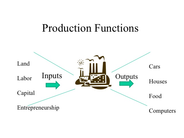
We are now going to focus on the what is backside the supply curve. Profits equal total acquirement minus full costs. Total revenue is equal to price times quantity and nosotros examined their relationship in the elasticity section. This department focuses on the second part of the equation, costs.  In order to produce, we must employ resource, i.e., land, labor, upper-case letter, and entrepreneurship. What happens to output as more than resources are employed?

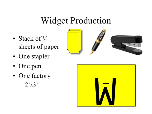
We tin can demonstrate the impact of adding more of a variable resources, say labor, to a fixed amount of capital and see what happens to output. For demonstration purposes in economics, we often make widgets, which is really any hypothetical manufactured device. Our widget volition be made taking a quarter canvas of paper, folding it in half twice then stapling it and writing the letter Westward on it.  If you have a large family, you can practise this as a Family Home Evening activeness; otherwise you tin just read along to see the results.  The inputs are a stack of quarter sheets of newspaper, one stapler, one pen, and a two' x 3' sail of poster board which represents your factory wherein all production must take identify. Each round is a sure amount of fourth dimension, say 40 seconds.

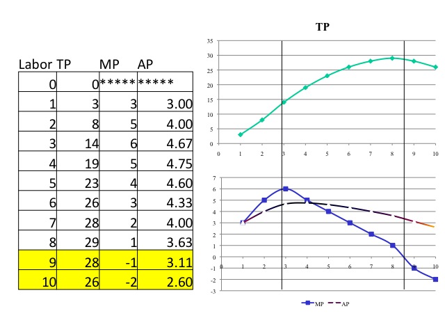
What will exist the output level of widgets as more than labor is added?  With zero workers, nothing gets produced. With one worker, the worker must fold the paper, staple it, and write the Due west. Doing all of these tasks by himself, our first worker is able to produce three widgets.

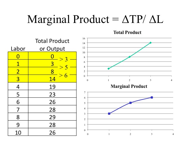
Marginal Product

Total product is but the output that is produced by all of the employed workers. Marginal product is the additional output that is generated by an additional worker. With a second worker, product increases by 5 and with the third worker information technology increases by 6. When these workers are added, the marginal product increases. What factors would cause this?  Equally more than workers are added, they are able to divide the corresponding tasks and specialize. When the marginal product is increasing, the total production increases at an increasing rate. If a business is going to produce, they would not desire to produce when marginal product is increasing, since by adding an boosted worker the cost per unit of output would be declining.

In The Wealth of Nations, Adam Smith wrote virtually the advantages of the segmentation of labor using the instance of a pin maker.  He pointed out that an private not educated to the business organisation could scarce make ane pin a day and certainly not more than twenty. Merely the concern of pivot making is divided up into a number of peculiar trades and each worker specializes in that trade. "One man draws out the wire, another straights it, a third cuts information technology, a 4th points information technology, a fifth grinds it at the top for receiving the head; to make the head requires 2 or iii singled-out operations; to put it on, is a peculiar business, to whiten the pins is some other; it is fifty-fifty a merchandise by itself to put them into the paper; and the important business organization of making a pin is, in this manner, divided into about 18 distinct operations, which, in some manufactories, are all performed past distinct easily, though in others the aforementioned human will sometimes perform ii or iii of them." As a outcome, these 10 people are able to produce upwards of xl-8 thousand pins in a day.

Reference: http://www.econlib.org/library/Smith/smWN1.html#B.I,%20Ch.1,%20Of%20the%20Division%20of%20Labor

Diminishing Returns

At some point, diminishing marginal returns sets in and the marginal product of another worker declines. As more than workers are added, the capital, i.e., factory size, stapler and pen become more than deficient. The law of diminishing marginal returns states that equally successive amounts of the variable input, i.due east., labor,  are added to a stock-still amount of other resources, i.e., capital,  in the product procedure the marginal contribution of the additional variable resource will eventually decline.  Every bit the marginal production begins to fall merely remains positive, full product continues to increment but at a decreasing rate. As long every bit the marginal production of a worker is greater than the average production, computed by taking the full product divided by the number of workers, the average product will rise. For students, it is often easiest to remember when y'all call back about your class point average. If your g.p.a. for this semester, i.e., your marginal g.p.a.,  is greater than your cumulative one thousand.p.a., i.e., your average g.p.a., so your average m.p.a. volition rise. Only if your chiliad.p.a. this semester is lower than your cumulative grand.p.a., so your cumulative thou.p.a. will autumn. Thus the marginal production will always intersect the boilerplate production at the maximum average production.

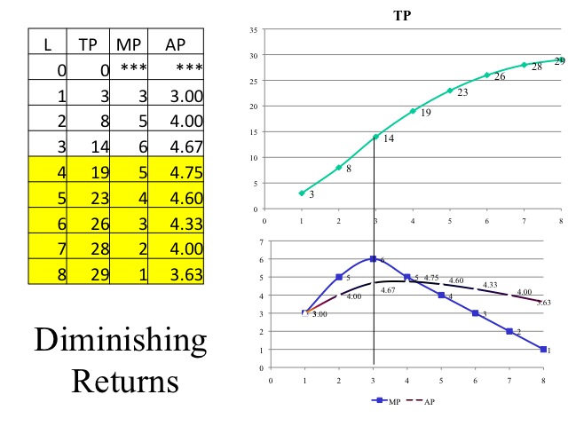
There may even come a point where adding an additional worker makes things and then crowded that full production begins to fall. In this case the marginal product is negative.  In our example, adding the ninth and tenth worker yields lower output than what was produced with only eight workers.

So how many workers should be employed?  We know that we would non stop in the region where marginal product is increasing and nosotros would non produce in the region where marginal product is negative.  Thus nosotros will produce where marginal product is decreasing but positive, merely without looking at the costs and the price that the output sells for, we are unable to determine how many workers to employ.

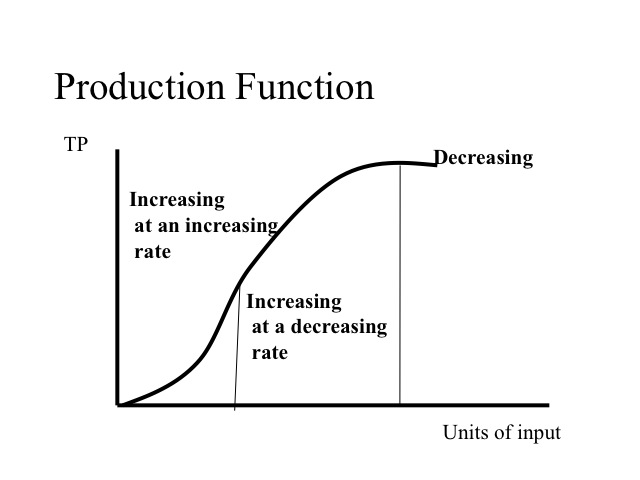
A production function shows the output or full production as more than of the variable input, in our example labor is added. The function shows the regions of increasing marginal product, decreasing marginal product, and negative marginal product.

Practice

Residential construction crews are often iii to eight people depending on the blazon of work.  Think of what factors would cause increasing and decreasing marginal productivity in construction. Think of another industry and what would exist the ideal number of workers?

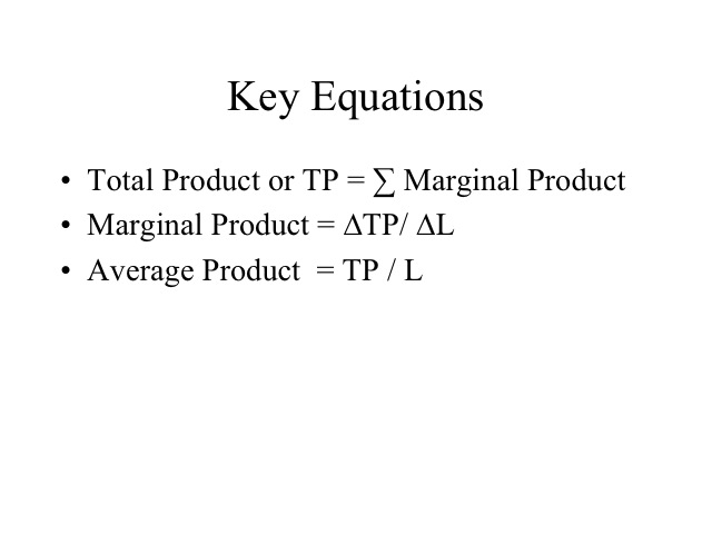
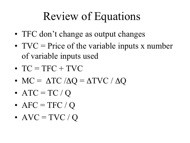
Key Equations

---

Section 02: Short Run Costs

Accounting vs. Economics

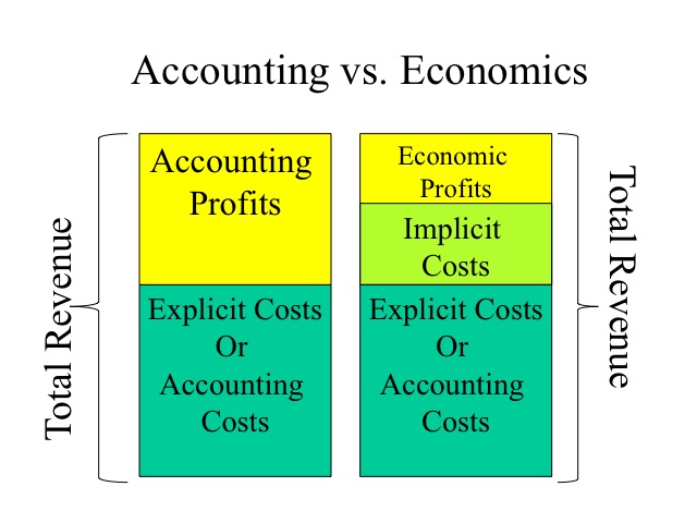
Recall that explicit costs are out-of-pocket expenses, such as payments for rent and utilities, and implicit costs reflect the opportunity costs of not employing the resource in the side by side best option.  Thus, the possessor of edifice doesn't accept to pay rent, but past using the building foregoes the opportunity of renting the building out to someone else.

Bookkeeping profits are calculating by subtracting the explicit costs from total revenue. Economical profits go a step farther and also decrease the implicit costs. Past including implicit costs, we can then determine if the resources are earning at least what could exist earned if employed in the next all-time choice. A normal profit is the minimum return to maintain a resource in its current utilise. If a business firm is earning zip economic profit would they still stay in business? A business firm that is earning a zero economic is earning a normal profit and there is no incentive to move the resources to another use, since the amount that they are earning is equal to the return that could be earned elsewhere.

Practice

Using the information beneath, compute the explicit and implicit costs, the accounting and economic profits.  And so explain what will happen in this industry and why.

Total Revenue  $600,000

Cost of materials  $200,000

Wages to employees  $250,000

Foregone wage      $100,000

Foregone rent and interest    $80,000

The explicit costs would be the out-of-pocket expenses of materials and employee wages: 200,000 + 250,000 = $450,000. The implicit costs are the foregone opportunities, in this instance the wage the possessor is giving up by working in her concern instead of working elsewhere and the foregone rent and involvement that could exist earned by the building and money tied upwardly in the company - $100,000 + $80,000 = $180,000.  The bookkeeping profit is $150,000 computed by taking the full revenue $600,000 less the explicit costs $450,000.  Subtracting the additional $180,000 of implicit costs leaves an economic profit of negative $30,000. Although the business organisation possessor is earning an accounting turn a profit of $150,000, her economic profit is negative pregnant that she could earn more than by shutting down the business and employing the resources in their next best alternative. Thus if this loss continues, we would conceptualize the owner would exit this business.

Fixed and Variable Costs

In the short run, at least 1 of the inputs or resources is stock-still. Fixed costs are those that do not alter equally the level of output changes. Variable costs are those costs that alter as output changes. Fixed costs can exist quite large. In the airline industry, for example, fixed costs range from twoscore to 70 pct of total costs. Thus during the week of September 11, 2001 when commercial flights were grounded, the airlines still incurred substantial costs fifty-fifty though they were not operating.   These fixed costs included items such as insurance, depreciation on equipment, taxes, and involvement on their loans.  Since they were not operating, all the same, variable costs such as jet fuel, meals on board, and wages to hourly employees were non incurred.

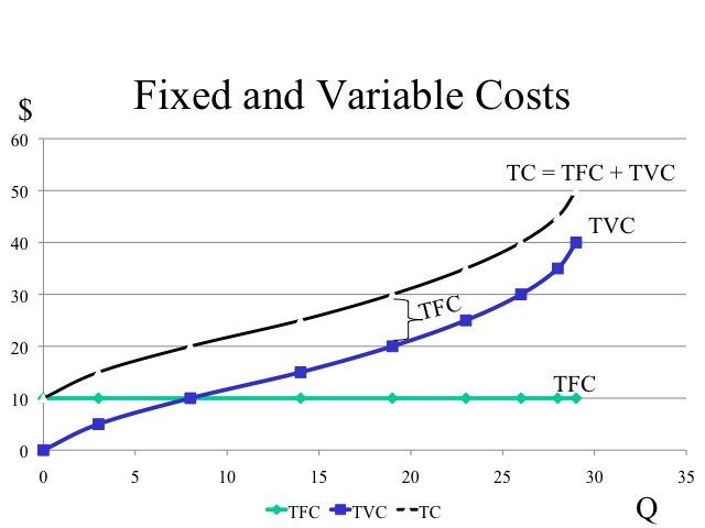
Since fixed costs do not change as output changes, the full fixed cost line is flat at the level of fixed price. If no production takes identify, variable costs are nix. As production increases, total variable costs increase at a decreasing rate, since the marginal product for each additional worker is increasing. With diminishing marginal production, the total variable cost increases at an increasing rate. Total costs is the sum of total fixed costs and full variable costs, thus full toll begins at the level of fixed costs and is shifted upwardly above the full variable price past the corporeality of the fixed toll.

Reference: http://www.accenture.com/Global/Research_and_Insights/By_Industry/Airline/AirlinesOutsourcing.htm

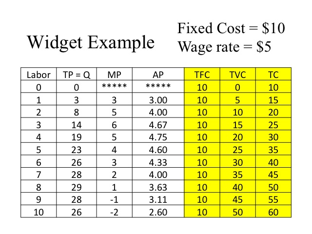
In our widget example, we will assume that the fixed cost for the stapler, pen, and "manufactory" is $ten and the cost of each worker hired is $5 per worker. Since fixed costs are constant, the firm incurs $x regardless of the level of output. Labor is the only variable toll computed by $5 times the number of workers. When we talk over costs, we are going to refer to our output as quantity denoted past a Q, instead of full product, denoted past the TP.

Equations

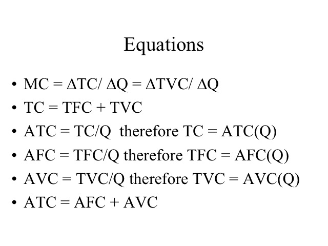
We can as well evaluate costs looking at the marginal costs and average costs. Marginal cost is the change in full cost divided past the change in output. Since fixed costs do not change with output, marginal toll can also be computed by dividing the modify in full variable toll by the change in quantity. If the equation, TC = TFC and TVC is divided by quantity, we get the average of each item, i.due east., average full cost equals boilerplate fixed costs plus average variable cost.

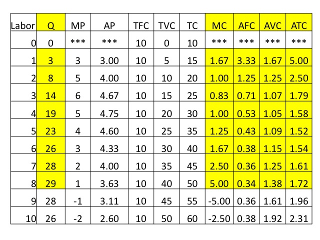
Using our widget instance, nosotros compute the  MC, AFC, AVC, and ATC. Annotation that we did not compute the marginal or average values at goose egg output.

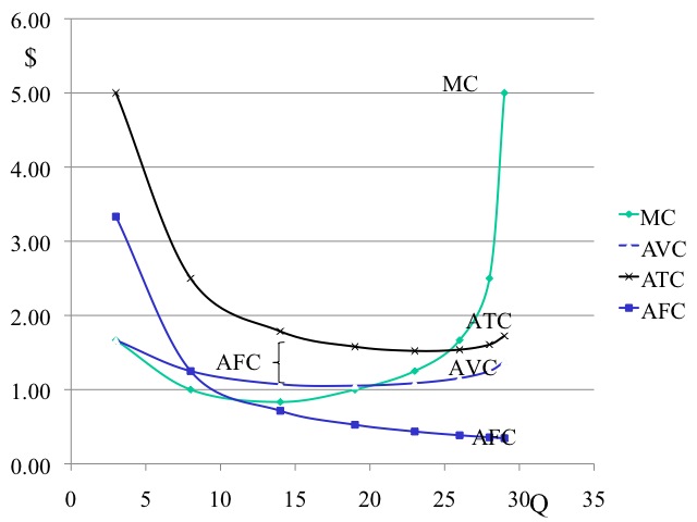
It is often easier to see important relationships when we graph the results for ATC, AVC, AFC, and MC. Keep in mind that we never produce where marginal production is negative, i.east., in our example we would never employ the ninth and tenth worker. And then we will graph only the output of ane to eight workers. We ofttimes do not graph the average fixed costs, considering average fixed toll is represented by the vertical distance between ATC and AVC.   However, in this example we will graph it so that yous tin can come across an important characteristic: since fixed costs don't alter with the level of output, average stock-still costs get smaller as more than quantity is produced, making the vertical distance between ATC and AVC smaller as output increases.  Another of import relationship can also be seen in these figures, and that is marginal cost intersects average variable and average total costs at their minimums.  Call back that a similar ascertainment was made for marginal product and average production, only in that case, marginal production intersected average product at its maximum.

Practice

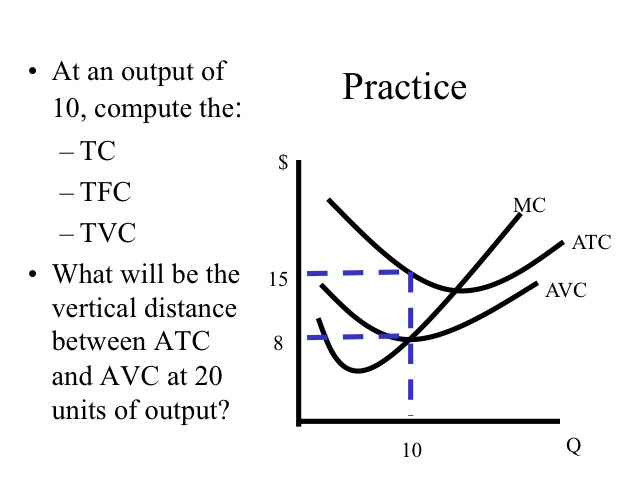
1. At an output of x, compute the (a) TC, (b) TFC, and (c) TVC.

2. What would be the vertical distance between ATC and AVC at 20 units of output?

Answers

Total Toll = ATC*Q = $xv*x = $150

Total Variable Toll = AVC*Q = $eight*10 = $eighty

The vertical distance between ATC and AVC is AFC, so TFC = AFC*Q = $7*10 = $seventy

If the total stock-still toll is $lxx then at xx units of output, the vertical altitude between ATC and AVC which is the AFC would be $3.50.

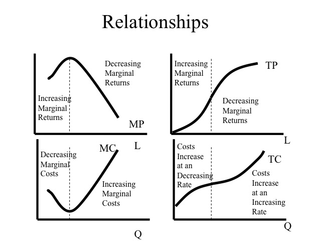
Relationships

Some of import relationships exit between the productivity measures (TP, AP, and MP) and the cost measures.  These relationships result from how productivity determines costs. Consider, for example, when a business concern adds i more worker who causes productivity to ameliorate.  This would mean that output is increased more for this worker than for previous workers!  On the margin, what practise you call up will happen to the additional price with respect to output?   Clearly the cost of that additional output will be lower because the house is getting more output per worker.  This results provides an interesting relationship between marginal cost and marginal product.  When marginal product is at a peak, then marginal cost must be at a minimum.  This will ever concord true, and as a result, marginal toll is the mirror prototype of marginal product. When marginal product is rising, the marginal cost of producing another unit of output is declining and when marginal product is falling marginal cost is ascent. Similarly, when average product is rising, boilerplate variable cost is falling, and when average product is falling, average variable cost is ascension (since average product corresponds the variable input changing, this important relationship exists with average variable cost and Non average total cost). Finally, when full product is increasing at an increasing rate the full cost is increasing at a decreasing charge per unit. When total product is increasing at a decreasing rate, the total price is increasing at an increasing rate.

Exercise

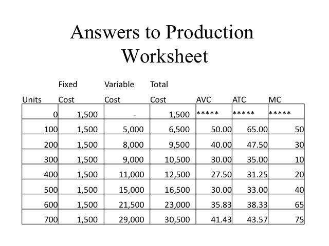
1. Complete the following worksheet. Utilise the equations beneath to help yous consummate the worksheet.

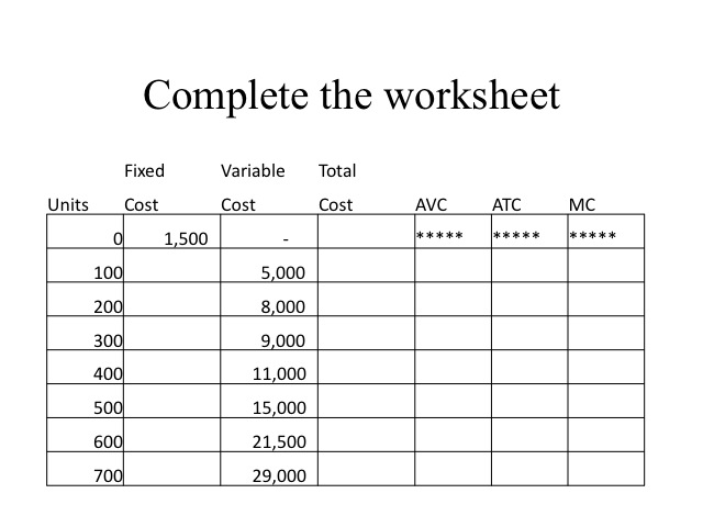
Answers to Production Worksheet

---

Section 03: Long Run Costs

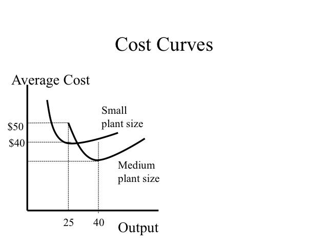
Cost Curves

The long run is that period of time that would permit all inputs or resources to become variable. In the long run, at that place are no fixed costs and a firm tin can decide the amount of each input. Think of a business concern just starting and they could determine the building size, the corporeality of equipment, the number of workers, etc. What would be the ideal quantity of each input?

Up until now, we have been because costs in the short-run, i.due east. when at least one factor is stock-still.  At present we want to consider what happens to costs when all inputs are variable, i.e. the long-run.  Typically, the constitute size can merely be changed in the long-run, that is, it is often the last input to become variable.  In the long-run, we desire to select a plant size that gives us the lowest costs for our level of output. For example, let's assume nosotros tin build different sizes of a plant. If the desired output is just 25 units, then a small found is able to produce at a lower average cost ($40) than the medium size plant ($l). However, if our desired output is 40 units, so the medium size constitute is able to produce at a lower average price than the small plant. Businesses often face the challenge of knowing what quantity of inputs (i.e., building and equipment size) to purchase that will allow them to be competitive today given their electric current marketplace share, simply nonetheless be able to grow and be competitive in the futurity every bit market share expands.

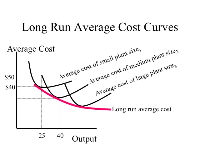
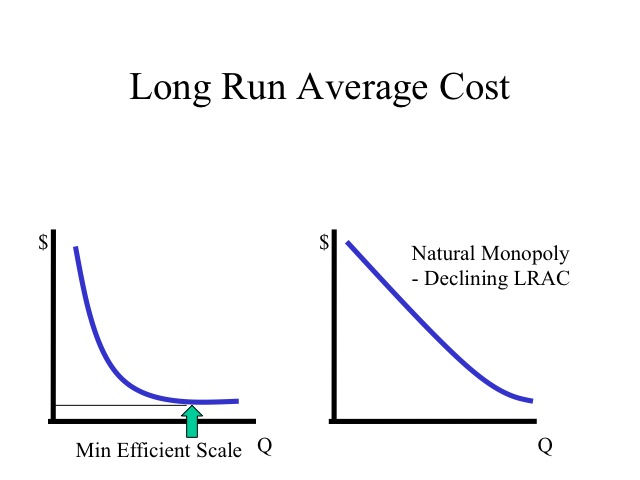
Assuming all factors are variable, the long run average cost bend shows the minimum average toll of producing any given level of output. The long-run average cost curve is obtained by combining the possible short-run curves (i.e. information technology is obtained by combining all possible establish sizes).  More particularly, it is a line that is tangent to each of the short run average toll curves. If increasing output reduces the per unit cost, the house is experiencing economies of scale (which ways larger found sizes have lower boilerplate full costs at their corresponding minimum points) . We typically come across this when plant sizes are minor.

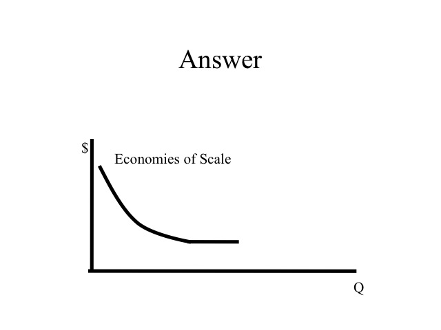
Economies of Calibration

This tin be explained based on a diversity of reasons.  As plant capacity increases, firms are able to specialize their labor and capital letter to a greater degree. Workers tin can specialize on doing a express number of tasks extremely well. Some other cistron contributing to economies of scale is the spreading out of the pattern and start up costs over a greater output amount.  For many products, significant costs are in  pattern and development. For example in the movie industry, the marginal cost of making a second re-create of a motion-picture show is nigh nix and as copies of the movie are produced, the average cost declines significantly.  Some picture makers will film the moving-picture show and its sequel at the same time to lower the per unit costs.

Equally larger quantities are produced, the inputs used tin be purchased in larger quantities and often at a lower per unit of measurement cost. The per unit of measurement cost when ordering a rail car or semi load of material is less than when purchasing the inputs in small quantities. Besides spreading the cost of placing the order over more units, reduces the per unit of measurement cost.

Reference:

http://world wide web.nytimes.com/2001/12/12/movies/gambling-picture-fantasy-lord-rings-shows-new-line-cinema-due south-value-aol.html?pagewanted=1

The cost structure of the industry determines the shape of its long run average toll curve. Some industries are able to attain the everyman per unit cost with a relatively pocket-sized plant size or scale of operation. Other industries exhibit a natural monopoly where the long run boilerplate cost curve continues to reject over the unabridged range of a product demand. In this type of an manufacture, it is hard for other firms to enter and compete since the existing firm has a lower per unit of measurement cost. The minimum efficient calibration is the constitute size  (or scale of functioning) that a firm must accomplish to obtain the lowest average cost or frazzle all economies of scales.

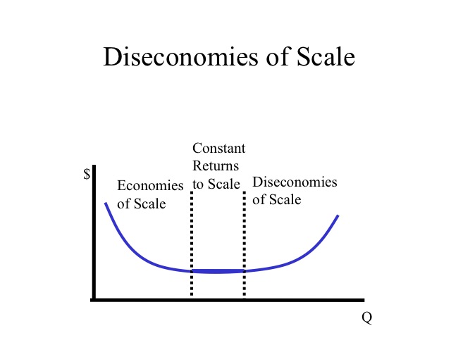
Diseconomies of Scale

The region where long run average costs remain unchanged as plant size increases is known as abiding returns to calibration. Diseconomies of scale occurs when average costs increment every bit plant size increases. As output increases the corporeality of cerise tape would increase equally it becomes necessary to hire managers to manage managers. Efficiency is lost as the size of the operation becomes too large.  If an auto manufacturer decided to produce all of its output at i location, remember of the size of the operation. Moving inputs into and out of the plant would raise costs significantly. Too, information technology would be difficult to find the needed workforce all in one urban center. Recognizing the diseconomies that could be, auto manufacturers accept instead chosen to produce their output at a number of different plants spread out throughout the globe.

Consider another case. Think of what it would toll to make your own machine. How many hours of blueprint would information technology take?  Equally you go to build the vehicle, think of the specialized tools that you would need to make the engine, frame, windows, ties, etc. Fifty-fifty if you built a auto for each fellow member of your family or every household in your boondocks, the cost per vehicle would enormous because at this calibration of operation, the caste of specialization is limited. Companies that do make cars produce thousands or even millions which allow them to specialize their capital and labor making the per unit of measurement cost significantly lower.

Think about this boosted example. Why tin can motion picture makers such as Disney or Pixar sell their movies that cost millions of dollars to brand for $20 each, while technical education videos that cost a few hundred thousand to produce volition sell for hundreds of dollars?

Pop movies will sell hundreds of thousands of copies, which allows the film makers to specialize their workforce and equipment since their calibration of operation will be significantly greater. On the other hand, technical didactics films price significantly less to produce merely only a few hundred copies will exist sold. Since their calibration of operation is small-scale, they are unable to gain the benefits of economies of scale that would permit them more than efficient use of labor and capital.

Economies of Telescopic

While economies of scale lowers the per unit of measurement cost as more of the same output is produced, economies of scope lowers the per unit cost as the range of products produced increases. For example, if a restaurant that provides lunch and dinner began to offer breakfast, the fixed costs of the kitchen equipment and the seating surface area could be spread out over a larger number of meals served decreasing the overall price per meal. Besides a gas station that already must have a service bellboy and building can lower the per unit cost by providing convenience store items such as drinks and snacks. Since the toll of producing or providing these products are interdependent, providing both lowers the toll per unit of measurement.

riosyoughbou.blogspot.com

Source: https://courses.byui.edu/econ_150/econ_150_old_site/lesson_06.htm

Share this post